Tutorial 04: Links and Data Collection
Tutorial Description
This tutorial covers how to:
Extracting state data of a particular link of a URDF object.
Extracting the mass of a particular link of a URDF object.
Storing data collected during simulation.
Creating a plot of the simulation data after the simulation has terminated.
Imports
To begin, we import the same modules for the same reasons as tutorial 00. We also include numpy and matplotlib.pyplot for data collection and visualization.
[1]:
from condynsate import Simulator as con_sim
from condynsate import __assets__ as assets
import numpy as np
import matplotlib.pyplot as plt
Building the Project Class
We now create a Project class with __init__ and run functions. In __init__ a pendulum is loaded using the same technique as tutorial 02. In run, we cover one way to collect data during the simulation that is available to users after the simulation completes. Futhermore, Project includes two additional functions, _add_data_point and plot_data. _add_data_point is what we use to collect and store simulation data during the simulation and plot_data is what we
use to generate a plot of those data after the simulation is complete.
[2]:
class Project():
def __init__(self):
'''
##################################################################
Differently that the previous tutorials, we have asked the
simulator to use a smaller time step than the default value of
0.01 seconds. Doing this will increase the simulation accuracy at
the expense of real-time execution time.
##################################################################
'''
# Create a instance of the simulator
self.s = con_sim(animation = False,
keyboard = False,
dt = 0.0075)
# Load the pendulum in the orientation we want
self.pendulum = self.s.load_urdf(urdf_path = assets['pendulum'],
position = [0., 0., 0.05],
yaw = 1.571,
wxyz_quaternion = [1., 0., 0., 0],
fixed = True,
update_vis = True)
'''
##################################################################
Differently that the previous tutorials, we set the initial
velocity instead of initial angle.
##################################################################
'''
# Set the initial angular velocity of the pendulum arm
self.s.set_joint_velocity(urdf_obj = self.pendulum,
joint_name = 'chassis_to_arm',
velocity = 1.571,
initial_cond = True,
physics = False)
def run(self, max_time=None):
'''
##################################################################
This run function does all the same basic functions as in
tutorial 02 but with the added functionality of data collection.
##################################################################
'''
# Create an empty dictionary of data to store simulation data
data = {'angle' : [],
'angle_vel' : [],
'KE' : [],
'PE' : [],
'time' : [],}
# Reset the simulator.
self.s.reset()
'''
##############################################################
To add a data point at the initial time step to the data
structure, we call the _add_data_point function.
##############################################################
'''
# Add the simulation data at the current time
data = self._add_data_point(data)
# Run the simulation loop until done
while(not self.s.is_done):
'''
##############################################################
Note that, compared to the previous tutorials, this time when
we call condynsate.simulator.step we store its return value.
condynsate.simulator.step gives a different return value
based on different situations. These return values are as
follows:
-4: Keyboard LOS indicating simulation step failure. No
simulation step taken. No further simulation steps are to
be taken. is_done flag is now true.
-3: User initiated simulation termination. No simulation step
taken. No further simulation steps are to be taken.
is_done flag is now true.
-2: User initiated pause is occuring. No simulation step taken.
paused flag remains true.
-1: User initiated pause has ended. No simulation step taken.
paused flag is now false.
0: User initiated simulation reset. No simulation step taken.
1: Normal and successful simulation step.
2: User initiated pause has started. Normal simulation step
taken. paused flag is now true.
3: max_time is now reached. Normal simulation step taken. No
further simulation steps are to be taken. is_done flag is
now true.
We want to keep track of these because if the simulation is
reset we will need to empty out all of the simulation data
that we have already collected, and if no simulation step was
taken, we don't want to collect any new data.
##############################################################
'''
# Take a single physics step.
ret_code = self.s.step(max_time = max_time)
'''
##############################################################
A ret_code greater than 0 indicates that a simulation step was
taken and the new data was created and can be added.
##############################################################
'''
# Add the simulation data at the current time if step was taken
if ret_code > 0:
data = self._add_data_point(data)
'''
##############################################################
A ret_code of 0 indicates the simulation was reset and we need
to reset the data also.
##############################################################
'''
# Reset data collection if sim is reset.
if ret_code == 0:
data = {'angle' : [],
'angle_vel' : [],
'KE' : [],
'PE' : [],
'time' : [],}
# Return the data
return data
'''
######################################################################
This function is what we use to collect data points during the
simulation. It collects joint and link state data, calculates
energies, and then appends these data to our data structure.
######################################################################
'''
def _add_data_point(self, data):
# Collect the state of the joint
state = self.s.get_joint_state(urdf_obj = self.pendulum,
joint_name = 'chassis_to_arm')
# Extract angle and angular velocity of the joints
angle = state['position'] * 57.296
angle_vel = state['velocity'] * 57.296
'''
##################################################################
To collect the state of a specific link in a URDF object we call
condynsate.simulator.get_link_state. This works for either the
base link or any children links and takes the following
arguments:
urdf_obj : URDF_Obj
A URDF_Obj whose state is being measured.
link_name : string
The name of the link whose state is measured. The link
name is specified in the .urdf file.
body_coords : bool
A boolean flag that indicates whether the passed
velocities are in world coords or body coords.
It then returns:
state : a dictionary with the following keys:
'position' : array-like, shape (3,)
The (x,y,z) world coordinates of the link.
'roll' : float
The Euler angle roll of the link
that defines the link's orientation in the world.
Rotation of the link about the world's x-axis.
'pitch' : float
The Euler angle pitch of the link
that defines the link's orientation in the world.
Rotation of the link about the world's y-axis.
'yaw' : float
The Euler angle yaw of the link
that defines the link's orientation in the world.
Rotation of the link about the world's z-axis.
'R of world in link' : array-like, shape(3,3):
The rotation matrix that takes vectors in world
coordinates to link coordinates. For example,
let V_inL be a 3vector written in link coordinates.
Let V_inW be a 3vector written in world coordinates.
Then: V_inL = R_ofWorld_inLink @ V_inW
'velocity' : array-like, shape (3,)
The (x,y,z) linear velocity in world coordinates of
the link.
'angular velocity' : array-like, shape (3,)
The (x,y,z) angular velocity in world coordinates of
the link.
##################################################################
'''
# Retrieve the state of the mass at the end of the rod
state = self.s.get_link_state(urdf_obj = self.pendulum,
link_name = 'mass',
body_coords = True)
'''
##################################################################
To collect the mass of a specific link in a URDF object we call
condynsate.simulator.get_link_mass. This works for either the
base link or any children links and takes the following
arguments:
urdf_obj : URDF_Obj
A URDF_Obj that contains that link whose mass is
measured.
link_name : string
The name of the link whose mass is measured. The link
name is specified in the .urdf file.
It then returns:
mass : float
The mass of the link in Kg. If link is not found,
returns none.
##################################################################
'''
# Get the mass of the mass
mass = self.s.get_link_mass(urdf_obj = self.pendulum,
link_name = 'mass')
'''
##################################################################
Finally, we use the collected link and joint data to add a single
data point to our data structure. This is done by appending the
calculated data to the end of its respective list.
##################################################################
'''
# Calculate the energy of the mass
height = state['position'][2]
vel = state['velocity']
KE = 0.5*mass*vel.T@vel
PE = mass*9.81*height
# Append the data to the list
data['angle'].append(angle)
data['angle_vel'].append(angle_vel)
data['KE'].append(KE)
data['PE'].append(PE)
data['time'].append(self.s.time) # This is how we get the current
# simulation time
# Return the new data list
return data
'''
######################################################################
The specifics of _plot_data are outside the scope of a condynsate
tutorial. See https://matplotlib.org/ for more information.
######################################################################
'''
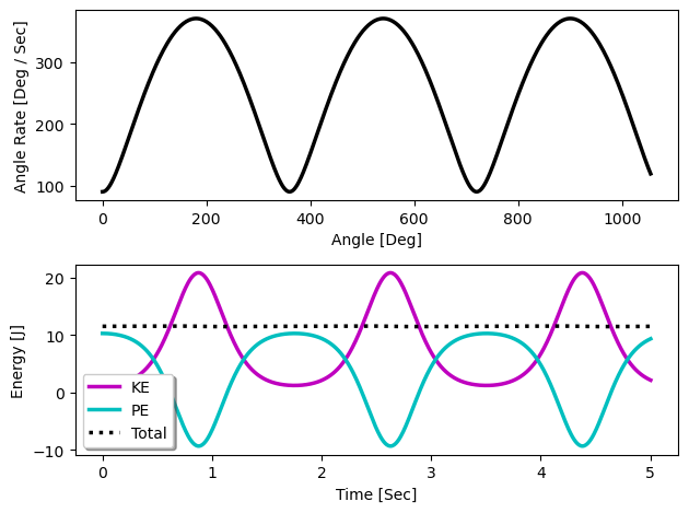
def plot_data(self, data):
# Make the plot and subplots
fig, (ax1, ax2) = plt.subplots(nrows=2, ncols=1)
# Plot the phase space
ax1.plot(data['angle'], data['angle_vel'], c='k', lw=2.5)
ax1.set_xlabel('Angle [Deg]')
ax1.set_ylabel('Angle Rate [Deg / Sec]')
# Plot the energy
ax2.plot(data['time'], data['KE'], label='KE', c='m', lw=2.5)
ax2.plot(data['time'], data['PE'], label='PE', c='c', lw=2.5)
total_E = np.array(data['KE']) + np.array(data['PE'])
ax2.plot(data['time'], total_E, label='Total', c='k', lw=2.5, ls=':')
ax2.legend(fancybox=True, shadow=True)
ax2.set_xlabel('Time [Sec]')
ax2.set_ylabel('Energy [J]')
# Figure settings
fig.tight_layout()
Running the Project Class
Now that we have made the Project class, we can test it by initializing it and then calling the run function. Remember to press the enter key to start the simulation and the esc key to end the simulation.
[3]:
# Create an instance of the Project class.
proj = Project()

# Run the simulation.
data = proj.run(max_time = 5.0)
You can open the visualizer by visiting the following URL:
http://127.0.0.1:7005/static/
[4]:
# Plot the data collected
%matplotlib inline
proj.plot_data(data)
Challenge
This tutorial is now complete. For an additional challenge, try creating a similar project but using the double pendulum provided in the condynsate default assests.